Building the Asset Lakehouse: Bronze, Silver, Gold for Maximo Objects
🎯 Who this is for: Data engineers building the actual pipeline past Part 2's extraction layer, analytics leads who need to know why a gold-layer number can be trusted, and any Maximo practitioner who has heard "we'll clean it in Databricks" and wants to know what that cleaning actually involves for WORKORDER, ASSET, and meter data specifically.
Series: Part 3 of 6 — MAS 9 + Databricks: Building the Maximo Data Lakehouse | Read time: 18 minutes
📖 Extraction Was the Easy Part
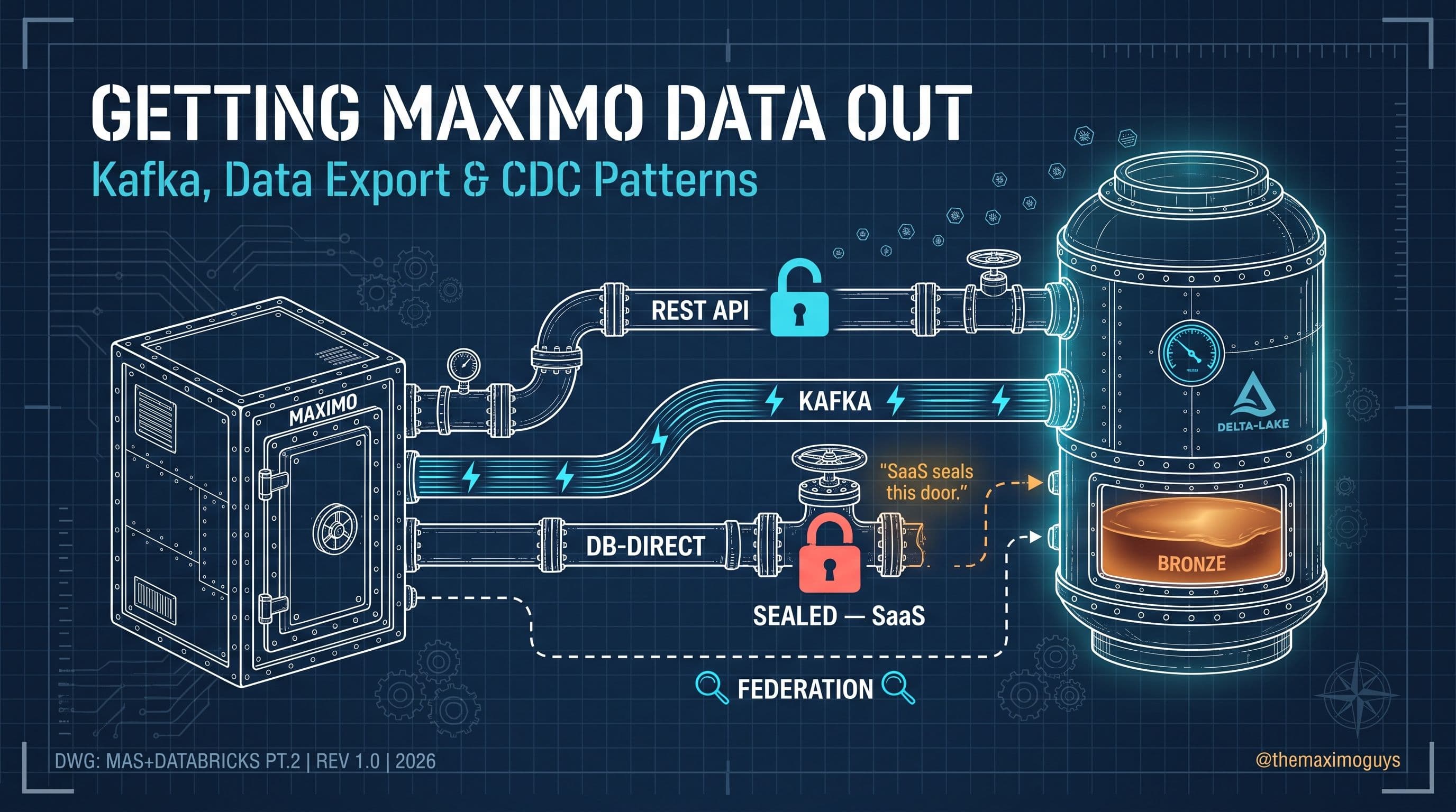
Part 2 of this series solved a real problem: getting Maximo data out of MAS 9 and into a bronze Delta table, using REST/JSON API extraction as the default, MIF over Kafka for near-real-time delivery, and an honest accounting of what "CDC" does and doesn't mean for a sealed SaaS database. That's a genuinely hard integration problem, and it's solved once you land raw MXAPIWO JSON in bronze.maximo_workorder_raw on a schedule.
It is also, on its own, worthless to an executive dashboard. A raw work order record has a wonum, a status code, an assetnum foreign key, and not much else that answers a business question. It doesn't know what asset class that asset belongs to, whether the site is a high-criticality plant, or what the failure code actually means in plain language. Answering "what's our maintenance cost trend for pumps at the Bedford site over the last two years" requires joining that raw work order against asset master data, location hierarchy, and failure history — and doing it consistently, every time, not as a one-off analyst query that gets a slightly different answer next month.
That's the gap this post closes. The medallion architecture — bronze, silver, gold — is the industry-standard answer to "how do you get from raw extracts to trustworthy business tables" in a Databricks lakehouse, and it maps unusually cleanly onto Maximo's own data model, because Maximo's Object Structures already group related business objects the way a silver-layer join would. This post works through that mapping table by table: what bronze actually holds, what real cleansing WORKORDER, meter, and PM data need in silver, how conformed dimensions keep "asset class" meaning the same thing across every downstream report, and which gold tables actually answer a reliability or cost question versus which ones are just restated bronze data wearing a nicer name.
💡 Key insight: The medallion architecture isn't an abstract data-engineering pattern bolted onto Maximo — it's the same three-tier idea Maximo's own Object Structures already embody at a smaller scale. MXAPIWO is Maximo's version of a silver-layer join (work order plus labor, materials, and failure data pre-assembled). This post extends that same idea past what one Object Structure can hold.📊 The Three Layers, Applied to Maximo
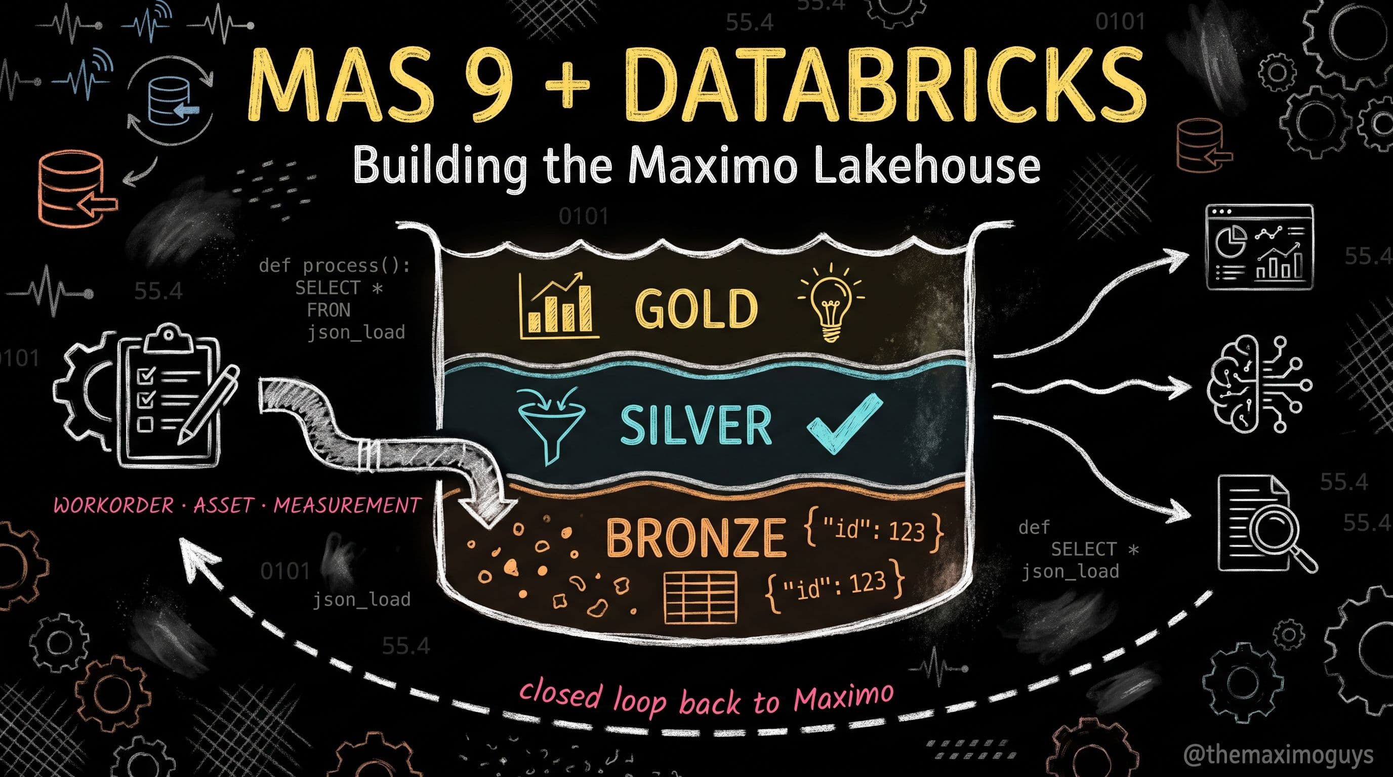
Before mapping individual tables, it's worth being precise about what each layer's job actually is, because the single most common lakehouse-build mistake is treating "clean the data" as one undifferentiated step instead of three layers with three different jobs. Databricks' own architectural guidance is specific here: bronze captures source data exactly as it arrived, silver applies "just-enough" cleansing to create a matched, merged, and conformed enterprise view, and gold applies the final business logic and data-quality rules that make a table consumption-ready for a dashboard or a report.
| Layer | Job | What changes about the data | Who queries it directly |
|---|---|---|---|
| Bronze | Land the raw extract | Nothing — append-only, schema mirrors the source JSON/CSV, plus ingestion metadata | Almost nobody; data engineers debugging a pipeline |
| Silver | Clean, join, conform | Deduplication, type casting, joins across related objects, meter-type-aware cleansing, slowly changing dimension handling | Data scientists building features, analysts who need row-level detail |
| Gold | Answer a business question | Aggregation, business rules, final data-quality gates, denormalized for read performance | Executives, Cognos/Power BI dashboards, ML training pipelines |
Notice the direction of travel: bronze is deliberately not clean, because a raw, unmodified copy is what lets you replay history when a silver-layer rule turns out to be wrong six months later. Gold is deliberately not row-level detail, because a table built for an executive KPI dashboard should not require the dashboard tool to re-derive an aggregation it could have gotten for free. Every mapping in this post respects that direction — resist the urge to "clean a little" in bronze or "keep raw detail" in gold, because both instincts erode the reason the three layers exist separately in the first place.
🥉 Bronze Layer — Landing Maximo Objects As-Is
Bronze's contract, restated from Part 2: hold the raw extract exactly as it arrived, whichever of the four extraction patterns produced it, with no transformation beyond adding ingestion metadata. For a Maximo lakehouse specifically, that means one bronze table per Object Structure or event source, landed via Auto Loader or Structured Streaming, never overwritten.
| Bronze table | Source | Format | Ingestion metadata added | |
|---|---|---|---|---|
| bronze.maximo_workorder_raw | MXAPIWO REST or Kafka Publish Channel | JSON → Delta | _ingested_at, _source_pattern (rest \ | kafka), _batch_id |
| bronze.maximo_asset_raw | MXAPIASSET REST | JSON → Delta | _ingested_at, _source_pattern | |
| bronze.maximo_locations_raw | MXAPILOCATIONS REST | JSON → Delta | _ingested_at, _source_pattern | |
| bronze.maximo_failurereport_raw | MXAPIFAILUREREPORT REST or Kafka | JSON → Delta | _ingested_at, _source_pattern | |
| bronze.maximo_measurement_raw | MXAPIMEASUREMENT REST or Kafka (IoT) | JSON/Avro → Delta | _ingested_at, _source_pattern, _meter_type (carried through, not derived) | |
| bronze.maximo_matusetrans_raw | MXAPIMATUSETRANS REST | JSON → Delta | _ingested_at, _source_pattern | |
| bronze.maximo_pm_raw | MXAPIPM REST | JSON → Delta | _ingested_at, _source_pattern | |
| bronze.maximo_historical_backfill | Data Export CSV (one-time) | CSV → Delta | _ingested_at, _backfill_source = "data_export" |
The _batch_id column on bronze.maximo_workorder_raw is worth calling out specifically, because it's what makes bronze genuinely replayable rather than just append-only in name. If a silver-layer join is discovered six months in to have a subtle bug — say, it's dropping work orders where FAILUREREPORT arrived a few minutes after WORKORDER in a Kafka-fed pipeline — you need to be able to say "replay every batch since the bug was introduced" without re-querying Maximo, which may no longer have that historical state available at the same granularity. A batch identifier tied to the ingestion job run makes that replay a WHERE _batch_id >= X filter instead of a re-extraction project.
-- Bronze: no cleansing, just landed exactly as it arrived
CREATE TABLE IF NOT EXISTS bronze.maximo_workorder_raw (
  wonum STRING,
  description STRING,
  status STRING,
  assetnum STRING,
  siteid STRING,
  changedate TIMESTAMP,
  worktype STRING,
  raw_payload STRING,          -- full JSON, in case downstream needs a field not yet promoted to a column
  _ingested_at TIMESTAMP,
  _source_pattern STRING,
  _batch_id STRING
)
USING DELTA
PARTITIONED BY (siteid);
Partitioning bronze by siteid rather than by ingestion date is a deliberate choice for Maximo data specifically — most silver-layer queries and most gold-layer marts filter or group by site first, and Delta Lake's file-pruning benefits from a partition column that matches the actual query pattern, not just the ingestion pattern. Keep the raw_payload column, too: promoting only the fields you think you need today is how a lakehouse ends up re-extracting from Maximo eighteen months later because a new gold table needs a field nobody promoted to bronze in year one.
💡 Key insight: If you find yourself deduplicating, joining, or casting types inside a bronze ingestion job, stop — that logic belongs in silver. Bronze's entire value is being a boring, unopinionated copy of the source; the moment it starts making judgment calls, you lose the ability to replay history when one of those judgment calls turns out wrong.
🥈 Silver Layer — Enriching Work Orders With Real Context
This is where a raw work order record becomes something a reliability engineer or a cost analyst can actually use, and it's the single highest-value silver table in the entire lakehouse, because nearly every gold-layer mart in this series traces back to it.
The WORKORDER-to-ASSET-to-LOCATIONS-to-FAILUREREPORT join
A raw bronze.maximo_workorder_raw record carries assetnum and siteid as foreign keys, but not the asset's class, criticality rating, or location hierarchy — and it doesn't carry failure-code detail unless the Object Structure was configured to nest it. The silver enrichment join assembles all of it into one record:
CREATE OR REPLACE TABLE silver.work_orders_enriched AS
SELECT
  wo.wonum,
  wo.siteid,
  wo.status,
  wo.worktype,
  wo.changedate,
  a.assetnum,
  a.description       AS asset_description,
  a.assettype         AS asset_class,
  a.priority           AS asset_criticality,
  loc.location,
  loc.description       AS location_description,
  loc.parent_location,
  fr.failurecode,
  fr.problemcode,
  fr.causecode,
  fr.remedycode,
  lab.actlabhrs,
  lab.actlabcost,
  mat.actmatcost,
  (COALESCE(lab.actlabcost, 0) + COALESCE(mat.actmatcost, 0)) AS total_actual_cost
FROM bronze.maximo_workorder_raw wo
LEFT JOIN silver.dim_asset a
  ON wo.assetnum = a.assetnum AND wo.siteid = a.siteid
LEFT JOIN silver.dim_location loc
  ON a.location = loc.location AND wo.siteid = loc.siteid
LEFT JOIN bronze.maximo_failurereport_raw fr
  ON wo.wonum = fr.wonum
LEFT JOIN (
  SELECT wonum, SUM(regularhrs + premiumhrs) AS actlabhrs, SUM(actlabcost) AS actlabcost
  FROM bronze.maximo_labtrans_raw GROUP BY wonum
) lab ON wo.wonum = lab.wonum
LEFT JOIN (
  SELECT wonum, SUM(linecost) AS actmatcost
  FROM bronze.maximo_matusetrans_raw GROUP BY wonum
) mat ON wo.wonum = mat.wonum
WHERE wo.status NOT IN ('CAN');  -- exclude cancelled work orders from cost/reliability analysis
Three details in this join matter enough to call out. First, the join to silver.dim_asset and silver.dim_location — not to bronze — is deliberate, and the conformed dimensions section below explains why: every other gold table in this series joins to the same two dimension tables, so a work order's "asset class" and a failure-prediction table's "asset class" are guaranteed to agree. Second, the labor and material subqueries aggregate at the work-order level before joining, because a work order can have many labor transactions and many material-use transactions, and joining at the raw transaction grain would fan out the row count and double-count cost — a mistake that's easy to make and produces cost numbers that are silently 3-4x too high. Third, excluding cancelled work orders happens here, in silver, not in every downstream gold query — that's what "just-enough cleansing" means in practice: apply a business rule once, in the layer built for it, instead of repeating a WHERE status != 'CAN' in every report that touches work orders.
💡 Key insight: The most common silver-layer bug in a Maximo lakehouse isn't a missing join — it's joining at the wrong grain. Labor and material transactions are one-to-many against a work order; joining them directly instead of pre-aggregating silently multiplies cost totals. Always ask "what's the grain of this table relative to what I'm joining it to" before writing the join.
🌡️ Silver Layer — Meter and Sensor Data, Cleaned the Maximo Way
Meter and sensor cleansing gets talked about in generic data-engineering terms — "time-align, remove outliers" — but Maximo's own Meters application already defines specific reading semantics that a generic outlier filter will get wrong if it ignores them, and getting this wrong produces a failure-prediction model trained on garbage.
Meter types dictate the cleansing rule
Maximo's Assets application lets you associate a meter with an asset as one of three types, and the type is not cosmetic — it changes what "clean" means for that meter's readings:
| Meter type | What it measures | Cleansing consideration |
|---|---|---|
| Continuous | Cumulative usage — runtime hours, odometer miles, cycle counts | Reading Type is Delta (incremental) or Actual (cumulative); Actual readings can legitimately roll over to a lower value, and Maximo's own Rollover flag marks this — a silver job that treats every value decrease as bad data will discard valid readings |
| Gauge | Point-in-time measurement — pressure, temperature, vibration amplitude | No accumulation logic; time-align to a common interval and apply straightforward range/null checks |
| Characteristic | Non-numeric condition — a text-based status or grade | No numeric cleansing at all; deduplicate on timestamp and validate against the configured domain of allowed values |
For continuous meters specifically, Maximo also lets an administrator configure an Average Calculation Method — All (use every reading), Sliding Days or Sliding Readings (use a rolling window), or Static (a fixed average that never recalculates) — and a silver job computing a derived "average daily usage" feature for an ML model should replicate whichever method the asset is actually configured with, not assume one uniformly. Getting this wrong doesn't crash the pipeline; it just quietly trains a remaining-useful-life model on a usage-rate feature that doesn't match what the asset's own configuration says usage looks like.
# Silver: meter-type-aware cleansing, not a generic outlier filter
from pyspark.sql import functions as F
from pyspark.sql.window import Window

readings = spark.table("bronze.maximo_measurement_raw")

continuous = readings.filter(F.col("_meter_type") == "CONTINUOUS")
w = Window.partitionBy("assetnum", "meter").orderBy("reading_date")

continuous_cleaned = (
    continuous
    # A lower reading is a legitimate rollover if Maximo flagged it — not a data error to discard
    .withColumn("is_rollover", F.col("rollover_flag") == True)
    .withColumn("prev_reading", F.lag("reading_value").over(w))
    .withColumn(
        "is_suspect",
        # Flag only decreases that were NOT marked as a rollover
        (F.col("reading_value") < F.col("prev_reading")) & (~F.col("is_rollover"))
    )
    .filter(~F.col("is_suspect"))  # quarantine suspects, don't silently drop — see quality gate below
)

gauge = readings.filter(F.col("_meter_type") == "GAUGE")
gauge_aligned = (
    gauge
    .withColumn("reading_minute", F.date_trunc("minute", "reading_date"))
    .groupBy("assetnum", "meter", "reading_minute")
    .agg(F.avg("reading_value").alias("reading_value"))  # collapse sub-minute noise to a 1-minute grid
)
Time-alignment for gauge and sensor data — collapsing readings to a consistent 1-minute grid, as shown above — matters for a downstream reason beyond tidiness: cross-sensor correlation (vibration rising alongside temperature, the pattern a failure-prediction model actually looks for) only works if both signals are sampled on the same clock. Two sensors reporting on independent, unaligned schedules will show spurious lag or lead in a naive join that has nothing to do with the physical relationship between them.
🔧 Silver Layer — Inventory Transactions and PM Effectiveness
Two more silver tables round out the enrichment layer, and both answer a specific downstream gold question this series returns to.
Material usage, joined to demand and supply history
silver.inventory_demand joins raw material-use transactions against inventory balances and purchase-order receipts, because a reorder-point recommendation needs both sides — how fast an item is actually consumed and how long it takes to resupply:
| Silver table | Source joins | What it enables downstream |
|---|---|---|
| silver.work_orders_enriched | WORKORDER + dim_asset + dim_location + FAILUREREPORT + aggregated LABTRANS/MATUSETRANS | Cost rollups, reliability trends, work order intelligence |
| silver.sensor_aligned | MEASUREMENT, time-aligned per meter type, rollover-aware | Failure prediction features, anomaly detection |
| silver.inventory_demand | INVENTORY + MATUSETRANS (demand history) + PO receipts (supply history) | Reorder point recommendations, stockout risk scoring |
| silver.pm_effectiveness | PM completion records + subsequent FAILUREREPORT entries within a lookback window + MATUSETRANS/LABTRANS cost | PM optimization — which PM tasks actually prevent failures |
PM effectiveness — the join that actually answers "is this PM working"
silver.pm_effectiveness is worth a worked example because it's the join that answers a question a lot of Cognos reports can't: does completing this preventive maintenance task actually reduce subsequent failures, or is it busywork?
CREATE OR REPLACE TABLE silver.pm_effectiveness AS
SELECT
  pm.pmnum,
  pm.assetnum,
  pm.frequency,
  pm.lastcompletiondate,
  COUNT(fr.failurecode) AS failures_within_90_days,
  SUM(wo.total_actual_cost) AS reactive_cost_within_90_days
FROM bronze.maximo_pm_raw pm
LEFT JOIN silver.work_orders_enriched wo
  ON pm.assetnum = wo.assetnum
  AND wo.worktype = 'CM'   -- corrective maintenance work orders only
  AND wo.changedate BETWEEN pm.lastcompletiondate AND DATE_ADD(pm.lastcompletiondate, 90)
LEFT JOIN bronze.maximo_failurereport_raw fr
  ON wo.wonum = fr.wonum
GROUP BY pm.pmnum, pm.assetnum, pm.frequency, pm.lastcompletiondate;
A PM task with a consistent pattern of zero failures_within_90_days across many assets and many completion cycles is a strong candidate for a frequency reduction — it's doing its job with room to spare. A PM task that shows failures clustering shortly after completion, repeatedly, across the fleet, is a candidate for a scope or procedure review, not just a frequency change — the task is running on schedule but not actually preventing the failure mode it's supposed to catch. Part 4 of this series builds the ranked, fleet-wide version of this query as one of its five worked analytics use cases; this silver table is what makes that gold-layer ranking possible without re-deriving the join every time.
🧭 Conformed Dimensions — One Enterprise View of an Asset
Every silver join above references silver.dim_asset and silver.dim_location rather than joining directly against bronze.maximo_asset_raw. That's not a stylistic preference — it's the mechanism that keeps every gold table in this lakehouse agreeing with every other gold table about what an asset actually is.
A conformed dimension is a single, shared reference table that every fact table in a star-schema model joins against for a given business entity, so "asset," "site," or "craft" carries exactly one definition across the whole lakehouse. Databricks' own dimensional-modeling guidance is explicit that this is not a legacy data-warehouse pattern being awkwardly retrofitted onto a lakehouse — Delta Lake actively supports it, with identity columns for surrogate key generation, Delta's time-travel and constraint features standing in for classic slowly changing dimension (SCD) handling, and Unity Catalog's three-level namespace (catalog.schema.table) as the place a conformed dimension physically lives so every downstream table references the same object instead of a private copy.
-- dim_asset: a conformed dimension, SCD Type 2 for attributes that change over time
CREATE OR REPLACE TABLE silver.dim_asset (
  asset_sk BIGINT GENERATED ALWAYS AS IDENTITY,   -- surrogate key, stable even if Maximo's assetnum is reused
  assetnum STRING,
  siteid STRING,
  description STRING,
  assettype STRING,        -- asset class, used consistently across every gold table
  criticality STRING,      -- changes over time — reclassified assets need history preserved
  location STRING,
  __start_at TIMESTAMP,
  __end_at TIMESTAMP,
  __is_current BOOLEAN
)
USING DELTA;
Why this matters concretely: without a conformed dim_asset, it's entirely possible for gold.maintenance_cost_kpis to define "critical asset" using the raw ASSETTYPE field while gold.failure_predictions — built by a different analyst, six months later — defines it using a custom CLASSSTRUCTURE attribute instead. Both reports will look correct in isolation. Neither will agree with the other when a stakeholder asks "why does the cost report say we have 340 critical assets and the reliability report says 290," and tracking down that discrepancy after the fact costs far more than building one shared dimension up front would have. Applying __is_current and SCD Type 2 history to criticality specifically matters because an asset's criticality rating does change — a pump gets reclassified after a process change — and a gold-layer trend report needs to know what the criticality was at the time of a given work order, not just what it is today.
💡 Key insight: If you catch two gold tables computing the same business concept — "critical asset," "asset class," "active site" — with two slightly different SQL expressions, that's the signal a conformed dimension is missing, not a coincidence to shrug off. Fix it once in dim_asset, not in every query that touches criticality.🥇 Gold Layer — Marts for Reliability and Cost
Gold's job, restated: answer a named business question, using the conformed silver tables above, with the final aggregation and business logic already applied so a dashboard tool doesn't have to re-derive it. Two gold tables anchor this series' reliability and cost analytics, and both are cheap to build once silver.work_orders_enriched and silver.dim_asset exist.
Maintenance cost rollup, by asset class and site
CREATE OR REPLACE TABLE gold.maintenance_cost_kpis AS
SELECT
  wo.siteid,
  a.assettype AS asset_class,
  DATE_TRUNC('month', wo.changedate) AS cost_month,
  SUM(wo.total_actual_cost) AS total_cost,
  COUNT(DISTINCT wo.wonum) AS work_order_count,
  ROUND(SUM(wo.total_actual_cost) / NULLIF(COUNT(DISTINCT wo.wonum), 0), 2) AS avg_cost_per_wo
FROM silver.work_orders_enriched wo
JOIN silver.dim_asset a
  ON wo.assetnum = a.assetnum AND a.__is_current = true
GROUP BY wo.siteid, a.assettype, DATE_TRUNC('month', wo.changedate);
Reliability trends — MTBF and MTTR per asset class
CREATE OR REPLACE TABLE gold.asset_reliability_kpis AS
SELECT
  a.assettype AS asset_class,
  wo.siteid,
  DATE_TRUNC('quarter', wo.changedate) AS reliability_quarter,
  COUNT(DISTINCT wo.wonum) AS failure_count,
  -- MTBF: total operating days in the quarter / number of failures, per asset class
  ROUND(90.0 * COUNT(DISTINCT a.assetnum) / NULLIF(COUNT(DISTINCT wo.wonum), 0), 1) AS mtbf_days,
  -- MTTR: average actual labor hours per corrective work order, a proxy for repair duration
  ROUND(AVG(wo.actlabhrs), 2) AS mttr_hours
FROM silver.work_orders_enriched wo
JOIN silver.dim_asset a
  ON wo.assetnum = a.assetnum AND a.__is_current = true
WHERE wo.worktype = 'CM'
GROUP BY a.assettype, wo.siteid, DATE_TRUNC('quarter', wo.changedate);
Both tables share the same two joins — silver.work_orders_enriched to silver.dim_asset — which is the payoff of building the conformed dimension and the enriched work-order table once, correctly, rather than per-gold-table. Part 4 of this series takes this same pattern and extends it to inventory and PM-effectiveness gold marts with the full worked SQL; the pattern established here — narrow, single-question gold tables built on shared silver — is what makes each of those five use cases a short addition rather than a new pipeline.
💡 Key insight: A gold table that just restates bronze data with a friendlier column name isn't gold — it's bronze with a costume on. The test for a real gold table: does it answer a specific business question on its own, with the aggregation and business logic already applied, or does the consuming dashboard still have to do real work? If the dashboard still has to group, join, or compute a ratio, the aggregation belongs in gold, not in the BI tool.
🚦 Data Quality Gates — Before Bad Data Reaches Gold
Every join and cleansing rule above assumes the bronze data feeding it is structurally sound, and that assumption needs a checkpoint, not blind faith. The pattern that's become standard practice in medallion implementations is a quality gate between bronze and silver: declared rules that check schema conformance and null-critical-field violations, with failures quarantined into a separate table rather than silently dropped or, worse, silently let through.
from pyspark.sql import functions as F

bronze_wo = spark.table("bronze.maximo_workorder_raw")

# Declare the rules explicitly rather than hand-writing ad-hoc filters per pipeline
quality_checked = bronze_wo.withColumn(
    "_quality_flag",
    F.when(F.col("wonum").isNull(), "MISSING_WONUM")
     .when(F.col("assetnum").isNull() & F.col("siteid").isNull(), "MISSING_ASSET_AND_SITE")
     .when(F.col("changedate") > F.current_timestamp(), "FUTURE_CHANGEDATE")
     .otherwise("PASS")
)

good_records = quality_checked.filter(F.col("_quality_flag") == "PASS")
quarantined = quality_checked.filter(F.col("_quality_flag") != "PASS")

quarantined.write.format("delta").mode("append").saveAsTable("bronze.maximo_workorder_quarantine")

# A single bad row is a data-entry fluke; a large failing share is a source-system problem
fail_rate = quarantined.count() / max(quality_checked.count(), 1)
if fail_rate > 0.05:
    raise ValueError(f"Quarantine rate {fail_rate:.1%} exceeds 5% threshold — halting silver promotion")
The 5% threshold in that last block isn't an arbitrary number to copy verbatim — it's an illustration of a real principle: a single work order missing its assetnum is a data-entry mistake worth quarantining and moving past, but a batch where a third of records fail a key check almost always means something upstream broke (a schema change in Maximo, a bad Object Structure configuration, a partial Kafka outage), and letting that batch flow into silver and then gold produces a confidently wrong dashboard, which is worse than an obviously broken one. Set the actual threshold to match how much noise your specific tables tolerate — reference tables like ASSET should tolerate far less than a noisy IoT sensor feed.
⚠️ Common Mistakes Building the Medallion Layers
- Joining raw transaction tables at the wrong grain. Joining
LABTRANSorMATUSETRANSdirectly againstWORKORDERwithout pre-aggregating fans out the row count and silently inflates cost totals — always aggregate one-to-many children before joining them into an enriched fact table. - Treating every meter the same way. Applying a generic "flag decreasing values as bad" rule to continuous meters discards legitimate rollover readings; check
_meter_typeand the Rollover flag before applying any anomaly rule. - Skipping conformed dimensions until "later." Two gold tables built independently, months apart, without a shared
dim_asset, will define "critical asset" differently — and the discrepancy surfaces during a stakeholder review, not during development. - Cleaning in bronze. Deduplication, type casting beyond JSON parsing, and joins belong in silver. A bronze table that's already been "cleaned a little" can't serve as the replay source when a silver rule needs fixing later.
- Building one wide gold table instead of several narrow ones. A single "everything" gold table becomes a maintenance burden the moment two different reports need slightly different aggregation grains — purpose-built, single-question gold tables are cheaper to reason about and to fix.
- No quarantine path for failed quality checks. Silently dropping rows that fail a schema or null check hides the fact that something upstream is broken; a quarantine table with a fail-rate threshold turns a silent data-quality problem into a visible, actionable alert.
🔧 Practical Notes Before Part 4
- Build `silver.dim_asset` and `silver.work_orders_enriched` first. Nearly every gold table in this series — cost, reliability, PM effectiveness — joins against one or both; getting these two right early makes every subsequent gold table faster to build.
- Match cleansing effort to what each table actually needs. Meter data needs Maximo-aware reading-type logic; reference tables like
ASSETmostly need SCD handling; transactional tables need grain-aware aggregation before joining. - Set quarantine thresholds per table, not globally. A 5% failure tolerance that's reasonable for noisy sensor data is far too loose for a reference table like
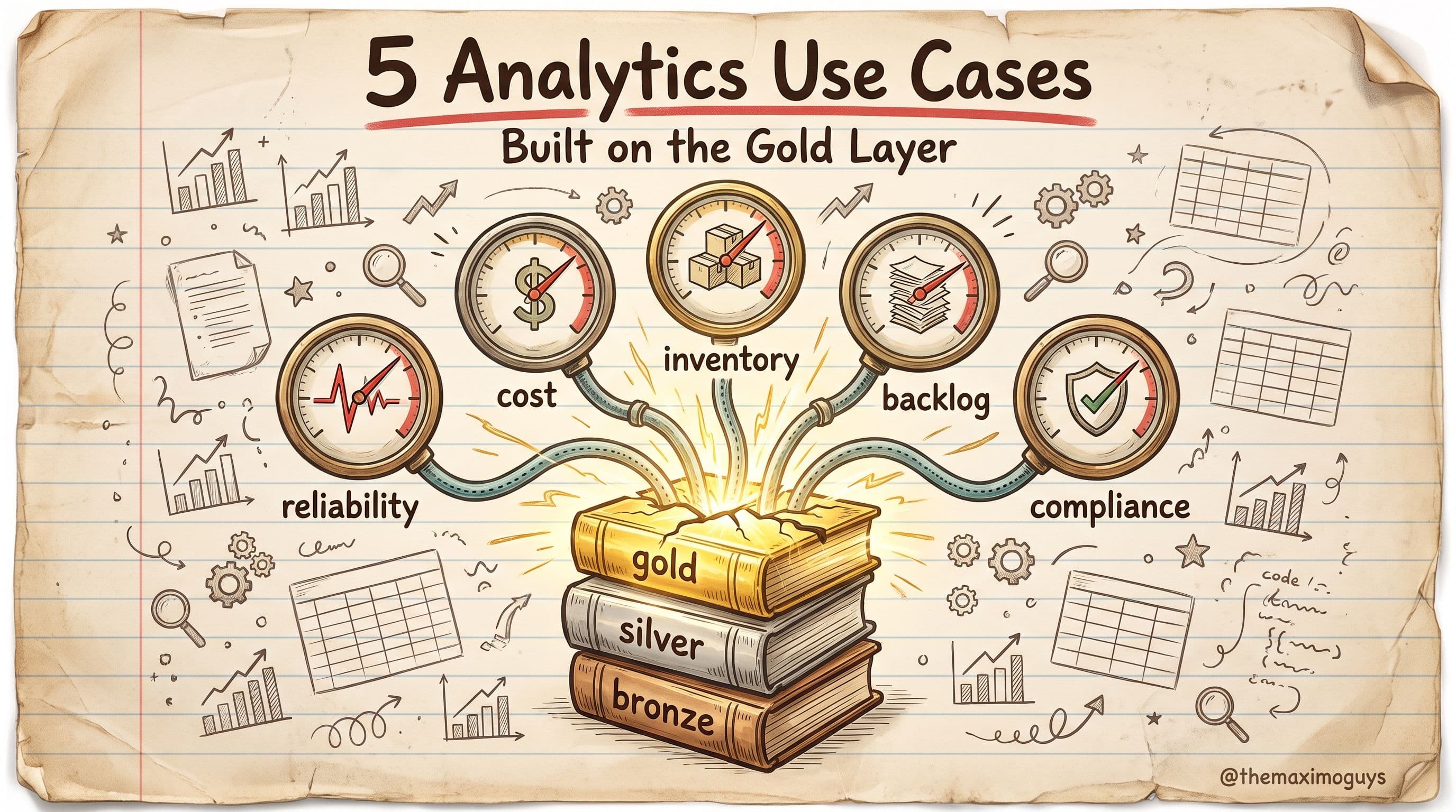
ASSETwhere a bad record should almost never happen. - Bring your gold-table wish list to Part 4 already scoped to one question each. Part 4 works through five concrete use cases — MTBF/MTTR trends, cost rollups, slow-moving inventory, backlog aging, PM compliance — and each is a narrow gold mart built on the silver tables from this post, not a new pipeline.
Key Takeaways
- Bronze is a strict, append-only landing zone — the raw extract from Part 2's four patterns, plus ingestion metadata, with no transformation, so any downstream rule can be replayed from source truth.
- Silver cleansing is table-specific — WORKORDER needs a real enrichment join against ASSET, LOCATIONS, and FAILUREREPORT; meter data needs Maximo's own reading-type and rollover semantics respected, not a generic outlier filter; PM records need a completion-to-failure join to measure effectiveness.
- Conformed dimensions prevent silent disagreement between gold tables —
dim_assetanddim_location, built once with SCD Type 2 history, keep "asset class" and "critical asset" meaning the same thing everywhere they're used. - A quality gate with a quarantine table and a fail-rate threshold turns silent bad-data problems into visible, actionable ones, and is what makes a gold-layer number trustworthy enough for an executive dashboard.
- Gold tables should each answer one named question, built from shared conformed silver tables — narrow and purpose-built beats one wide table trying to serve every report.
References
- Databricks — What is Medallion Architecture?
- Databricks on AWS — What is the medallion lakehouse architecture?
- Databricks — Lakehouse Data Modeling: Myths, Truths, and Best Practices
- Databricks — Loading a Data Warehouse Data Model in Real Time with the Databricks Lakehouse
- Databricks — The AUTO CDC APIs: Simplify Change Data Capture with Pipelines
- Maximo Secrets — New Features in MAS 9.0 and 9.1
Series Navigation
| Previous: | Part 2 — Getting Maximo Data Out |
|---|---|
| Next: | Part 4 — Five Analytics Use Cases |
About TheMaximoGuys: We help Maximo developers and teams navigate the move to MAS 9 with practical, no-hype guidance grounded in how the platform actually behaves.
Published by TheMaximoGuys | July 2026

 Surendra Katta