Reliability Metrics That Matter: MTBF, MTTR, Availability & PM Optimization
🎯 Who this is for: Reliability engineers and maintenance managers who need to measure whether a strategy is working — and use those numbers to tune PM intervals instead of guessing.
Series: Part 2 of 7 — MAS 9 Reliability Implementation Playbook | Read time: 19 minutes
📊 Why Metrics Are the Feedback Loop, Not a Scoreboard
In Part 1 you made decisions — one task type per failure mode. Metrics are how you find out whether those decisions were right, and they are the only honest basis for changing them. Without measurement, a reliability program is a set of opinions that ossify into policy. With it, the program becomes a control loop: you make a decision, you observe the failure history and downtime it produces, and you adjust.
That is the mental model to carry through this whole part. MTBF is not a number you report to look busy; it is the signal that tells you a PM interval is too long. MTTR is not a KPI for a slide; it is the lever that tells you availability can be won in the repair bay, not just in prevention. Metrics that are collected but never act back on the strategy are pure overhead. Everything below is oriented toward the action, not the report.
<aside>
💡 Key insight: The reliability metrics you compute in this part are produced by the exact objects you build in Part 3 and the feedback loop you close in Part 7. Failure reporting on the work order gives you the failure counts; meters give you operating time; labour transactions give you repair time. The metrics are the output of good data capture, which is why the spine has to come first.
</aside>
🧮 The Core Reliability Formulas
Here is the whole vocabulary in one table. Everything that follows is an application or a caveat of these.
| Metric | Formula | Applies to |
|---|---|---|
| MTBF (Mean Time Between Failures) | Total operating time ÷ number of failures | Repairable assets |
| MTTF (Mean Time To Failure) | Total operating time ÷ number of units | Non-repairable items |
| MTTR (Mean Time To Repair) | Total repair time ÷ number of repairs | Repairable assets |
| Availability (inherent) | MTBF ÷ (MTBF + MTTR) | Repairable assets |
| Failure rate λ | 1 ÷ MTBF | Constant-failure-rate regime |
| Reliability function | R(t) = e^(−λt) | Constant-failure-rate assumption |
| OEE (Overall Equipment Effectiveness) | Availability × Performance × Quality | Production equipment |
MTBF vs MTTF — the distinction that trips people up
The difference is not pedantry. MTBF is for things you repair and return to service — a pump, a motor, a conveyor. Its clock is "operating time between one failure and the next." MTTF is for things you replace rather than repair — a bearing, a seal, a bulb. Its clock is "operating time until the one failure it will ever have." Mixing them corrupts your analysis: computing "MTBF" for a consumable that is scrapped on failure produces a number with no physical meaning.
MTTR — decide what counts as repair time
MTTR is deceptively simple until you ask which clock. Pure "wrench time" (the time a technician is actively working) is a different number from "mean time to restore" (from failure detected to asset back in service, including waiting for parts, permits, and access). Both are legitimate; they answer different questions. For availability you generally want the restore clock, because a pump waiting three days for a seal is unavailable whether or not anyone is turning a wrench. In Maximo, wrench time comes from LABTRANS; the restore clock comes from work order status timestamps (from INPRG to COMP). Decide which you mean and be consistent, or your availability numbers will quietly drift.
🔢 A Fully Worked Calculation: A Fleet of Twelve Pumps
Numbers make this concrete. Suppose you run 12 identical process pumps and you are analyzing one year.
Given:
- Each pump ran, on average, 8,000 operating hours in the year (they are not 24/7 — there is standby rotation and planned downtime).
- Across the fleet, there were 18 failures in the year.
- Total repair time across those 18 events was 144 hours (from failure to restored).
Step 1 — Total operating time:
12 pumps × 8,000 h = 96,000 operating hours.
Step 2 — MTBF:
96,000 h ÷ 18 failures = 5,333 hours between failures (fleet average).
Step 3 — MTTR:
144 h ÷ 18 repairs = 8 hours mean time to repair.
Step 4 — Availability:
A = MTBF ÷ (MTBF + MTTR) = 5,333 ÷ (5,333 + 8) = 5,333 ÷ 5,341 = 0.9985 → 99.85%.
Step 5 — Failure rate λ:
λ = 1 ÷ MTBF = 1 ÷ 5,333 = 0.0001875 failures per hour (≈ 1.64 failures per pump-year of continuous running).
Step 6 — Reliability over a 720-hour month (constant-rate assumption):
R(720) = e^(−λt) = e^(−0.0001875 × 720) = e^(−0.135) = 0.874 → about an 87.4% chance a given pump survives a 720-hour run without failing.
<aside>
💡 Key insight: Availability of 99.85% looks reassuring — but the reliability function says each pump has a ~12.6% chance of failing in any given month of continuous running. High availability and mediocre reliability coexist when repairs are fast. That is exactly why you never manage on availability alone: it can hide a machine that fails constantly but recovers quickly.
</aside>
📈 Availability, and Why You Attack It From Both Sides
Look again at the availability formula: MTBF sits in the numerator and the denominator; MTTR sits only in the denominator. That structure has a strategic consequence.
You can raise availability by failing less often (↑ MTBF) or by recovering faster (↓ MTTR) — and the second is often cheaper.
In the worked example, halving MTTR from 8 hours to 4 hours moves availability from 99.85% to 99.925% — a small move because MTBF already dominates. But on a machine where MTTR is 40 hours and MTBF is 400 hours, availability is 400/440 = 90.9%; cut MTTR to 10 hours and availability jumps to 400/410 = 97.6% with no reliability improvement at all. On unreliable, slow-to-repair assets, the fastest availability win is in the storeroom, the kitting process, and the permit-to-work flow — not in more PMs.
This is why a mature reliability program invests in both: failure prevention (Parts 3–4) and the mean-time-to-restore levers (spares strategy, job-plan quality, standardized failure reporting so the next repair is faster). Maximo supports both — the failure hierarchy speeds diagnosis, and good job plans with pre-kitted materials cut restore time.
🛁 The Bathtub Curve
Why is age sometimes the right driver for maintenance and usually not? The bathtub curve is the picture.
 failure
  rate λ
    │\                                        /
    │ \      infant     useful life      wear-│out
    │  \    mortality   (constant λ)         /
    │   \  (λ falling)                      /
    │    \___________________________ _____/
    │         (random failures dominate here)
    └────────────────────────────────────────▶ age
burn-in design life end of life- Infant mortality (left): a decreasing failure rate. New or freshly repaired equipment fails early from manufacturing defects, installation errors, and — critically — maintenance-induced faults. This region is why intrusive PM can make things worse: every time you open an asset up, you reset it to the left of the curve.
- Useful life (middle): a roughly constant failure rate. Failures here are effectively random with respect to age. This is where most industrial equipment spends most of its life.
- Wear-out (right): an increasing failure rate. Genuine age-related degradation — the only region where a time-based PM based on age actually reduces failure probability.
The single most important thing the curve tells you: time-based PM only helps in the wear-out region. Applied in the useful-life (random) region, a calendar PM cannot lower the failure rate — and, by returning the asset to the infant-mortality zone, it can raise it.
🎯 The Nowlan & Heap Finding: The Critical Insight
Here is the fact that should reshape your PM program. The Nowlan & Heap studies of the 1970s — the foundational research behind RCM, conducted on commercial aircraft fleets — found that only about 11% of failure modes exhibit an age-related (wear-out) pattern. The other ~89% are random or infant-mortality dominated. Later studies across other industries broadly confirmed the pattern.
The studies identified six failure-rate patterns; only three show any "wear-out" behaviour that a calendar interval could catch, and together the age-related ones account for roughly 11% of modes:
| Pattern | Shape | Age-related? | Right response |
|---|---|---|---|
| A — Bathtub | infant + constant + wear-out | Partly | PM at wear-out; watch burn-in |
| B — Wear-out | constant then rising | Yes | Time-based PM |
| C — Gradual rise | steadily increasing | Yes | Time-based PM / CBM |
| D — Initial rise then constant | rises then flat | No (net) | CBM / RTF |
| E — Constant (random) | flat throughout | No | CBM / RTF / failure-finding |
| F — Infant mortality then constant | high then flat | No | Fix quality; CBM / RTF |
Patterns D, E, and F — the large majority — are not age-related. For those modes, adding a time-based PM is spending money to move a number that will not move.
<aside>
⚠️ Watch out: Pattern F (infant mortality then constant) is the most counter-intuitive and the most common on complex electronics and freshly overhauled equipment. For F modes, more intrusive maintenance actively increases failures by repeatedly re-introducing infant mortality. The correct response is better installation and commissioning quality, then run-to-failure or CBM — not a shorter PM interval.
</aside>
🔧 PM Optimization: A Concrete Method
The Nowlan & Heap finding is not academic — it is an operating instruction. PM optimization is the disciplined act of moving your program toward the ~11% and off the ~89%. Here is a method you can run against your own Maximo history.
Step 1 — Pull the evidence
For each PM (or each failure mode), extract from Maximo: the number of PM-generated work orders, the number of corrective work orders on the same asset/failure class, and the meter or calendar interval. Failure reporting (Part 3) gives you the corrective counts by problem/cause/remedy; the PM record gives you the interval; meters give you operating time.
Step 2 — Classify each PM into one of three buckets
| Evidence pattern | What it means | Action |
|---|---|---|
| PM runs, finds nothing, no corrective failures between PMs | Interval is conservative or the mode is not age-related | Extend the interval (or drop to CBM/RTF) |
| PM runs, corrective failures still occur between PMs | The mode is real but the interval is too long — or it is not age-related at all | Shorten if wear-out; switch task type if random |
| PM is intrusive and corrective failures spike right after each PM | Maintenance-induced infant mortality | Reduce intrusiveness; move to CBM or RTF |
Step 3 — Shift, don't just tune
The biggest gains come not from nudging intervals but from changing task type. A random-failure mode sitting on a monthly PM is a candidate to move to condition-based monitoring (a measurable signal, Part 3) or run-to-failure with a spare. That is where the ~89% goes.
Worked example — the PM that never finds anything
You have a monthly PM on a set of 40 non-critical exhaust fans: inspect and lubricate. A year of Maximo history shows 480 PM work orders, zero findings on 468 of them, and 12 corrective work orders — all for motor bearing failures that occurred regardless of the lubrication PM, scattered randomly across the year. Diagnosis: the lubrication PM is catching nothing (extend or drop it), and the real failure mode (bearing, random pattern E) is not age-related — so a shorter PM would not help. The optimized strategy: drop the monthly inspection to quarterly, and put the bearings on a simple vibration check (CBM) or run-to-failure with stocked spares. You have removed ~360 useless work orders a year and addressed the actual failure mode.
<aside>
💡 Key insight: The headline result of PM optimization is almost always fewer time-based PMs, not more — because you are pruning calendar tasks that fight random failures and replacing them with condition-based tasks that actually see the degradation. A program that only ever adds PMs has never been optimized.
</aside>
📉 OEE and the World Beyond Availability
Availability answers "was the machine able to run?" It does not answer "did it produce good output at rate?" Overall Equipment Effectiveness closes that gap:
OEE = Availability × Performance × Quality
- Performance captures speed losses — a line available but running below rated throughput.
- Quality captures scrap and rework — a line running but producing off-spec output.
A machine at 99% availability, 80% performance, and 95% quality has an OEE of 0.99 × 0.80 × 0.95 = 75.2% — a very different story from "99% available." For reliability engineers, OEE is the bridge to operations: it shows that reliability failures are only one of three loss buckets, and it keeps the conversation honest about where the money actually leaks.
🗺️ Where These Metrics Live in Maximo
None of this is theoretical in MAS 9 — every input is an object you already have.
| Metric input | Maximo source | Notes |
|---|---|---|
| Failure counts | Work order failure reporting (problem/cause/remedy), constrained by failure class | Part 3 builds the hierarchy that makes counts analyzable |
| Operating time | Meters (continuous, e.g. run hours) | Part 3; drives MTBF denominators and meter-based PM |
| Repair time (wrench) | LABTRANS labour transactions | Actual hours booked to the work order |
| Restore time | Work order status timestamps (INPRG → COMP) | The availability clock |
| Reported metrics | Manage KPIs, reports, and dashboards | Surface MTBF/MTTR/availability trends for review |
The takeaway: the quality of your metrics is bounded by the quality of your failure reporting and meter capture. Garbage free-text failure data (the thing Part 6 and Part 7 cleanse) produces garbage MTBF. This is the mechanical reason the spine has to be built and enforced before the metrics mean anything.
⚠️ Metric Gotchas
- Operating time ≠ calendar time. If you divide by calendar hours instead of operating hours, MTBF is inflated for anything that spends time on standby. Use continuous meters.
- Censored data. Assets that have not yet failed still carry information. Ignoring survivors biases MTBF downward. For rigorous work, use survival analysis, not a naive average — but a consistent naive MTBF is fine for tracking trends.
- Small samples lie. One pump with two failures gives an MTBF you should not bet a strategy on. Aggregate to the failure-class/fleet level (as in the twelve-pump example) before drawing conclusions.
- Chasing a single number. Managing to "improve MTBF" invites gaming (reclassifying failures as "not really failures"). Manage to the decision the metric informs, not the metric itself.
📋 Practical Notes: Building Your First Reliability KPI Set
- Start with three numbers per critical failure class: MTBF, MTTR, and corrective-vs-PM work order ratio. That trio drives every optimization decision above.
- Aggregate to failure class, not individual asset. Fleet-level numbers are statistically meaningful; single-asset numbers usually are not.
- Put the metrics on a quarterly review cadence (Part 7's Phase 5). Reliability metrics are a control loop, and a loop with no review is open.
- Tie every metric back to an action. For each KPI, write the one decision it informs — "if this MTBF trend flattens, extend the interval." A KPI with no attached decision is a vanity number.
- Trust the trend before the absolute. Your first MTBF numbers will be imperfect because the historical data is imperfect. The direction over quarters is what tells you the strategy is working.
Key Takeaways
- The core formulas are simple and interlocking: MTBF = operating time ÷ failures, MTTR = repair time ÷ repairs, and availability = MTBF ÷ (MTBF + MTTR).
- Availability is won from both sides — fewer failures (↑ MTBF) and faster recovery (↓ MTTR) — and on slow-to-repair assets, MTTR is often the cheaper lever.
- The bathtub curve explains why time-based PM only helps in the wear-out region; in the random-failure region it cannot lower the failure rate and can raise it.
- Only ~11% of failure modes are age-related (Nowlan & Heap) — most PM optimization is about moving modes off time-based PM, not adding more of it.
- Optimize from real Maximo history: extend where nothing fails, shorten where wear-out recurs, and shift random modes to CBM or run-to-failure.
References
IBM Official
- Maximo Manage — KPIs and reporting (IBM Documentation)
- Maximo Manage — Meters overview (IBM Documentation)
Standards & Community
- Nowlan & Heap — Reliability-Centered Maintenance (foundational RCM study)
- Maximo Secrets — Failure Codes and Failure Reporting
Series Navigation
| Previous: | Part 1 — Reliability Fundamentals: RCM, FMEA/FMECA & Task Types |
|---|---|
| Next: | Part 3 — Building the Reliability Spine in Manage |
About TheMaximoGuys: We help Maximo teams navigate the move to MAS 9 with practical, no-hype guidance grounded in how the platform actually behaves — from architecture and migration planning to the day-to-day work of configuring, extending, and running Maximo.
Published by TheMaximoGuys | July 2026

 Venkat Achanta